
Spectroscopy can feel intimidating at first, but absorbance measurements don’t have to be complicated.
This quick‑start guide walks through how to set up an absorbance measurement in OceanView without overthinking the process.
Quick Start: The Essentials
Short on time? These are the essential steps for a clean absorbance measurement.
- Set integration time so signal sits near the blue line
- Set boxcar and averaging to ~5
- Take light reference with light on and sample in place
- Take dark reference with light blocked or off
- Use autoscale to view absorbance clearly
- Save data using the gear and download icons
Jump Links
Use the links below to jump to the part of the setup you’re working on.
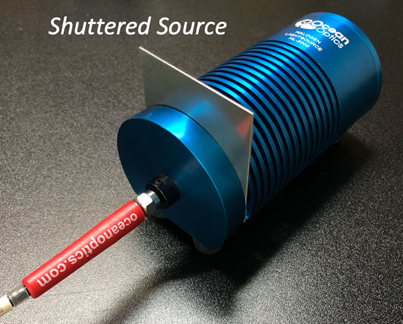
Hardware: What to Check First
You’re likely using a cuvette holder, probe, or some transmissive mount to measure your sample. Whatever your setup, make sure the basics are covered before opening the OceanView software.
- Fiber connections are tight between all components
- The optical path is stable and undisturbed
- You have a way to block or turn off the light source without disturbing the optical chain
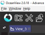
Open OceanView and Select Absorbance
Open OceanView and pick the Quick View option if prompted. If your spectrometer is recognized correctly, a live spectrum will appear along with a small status circle in the lower-right corner of the window.
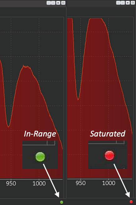
A green circle indicates the signal is within range. A red circle means the signal is saturated, which we will address next.
Select the Absorbance Wizard
Click the OceanView icon in the upper-left corner to open the Wizard menu and select the Absorbance.
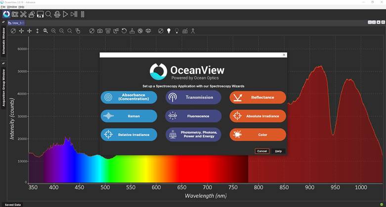
Select the first option, Absorbance Only, and click Next.
Expose the System to a Blank Sample
Turn on your light source and expose the system to what you consider your blank sample.
- For cuvettes or liquid vessels, this is usually distilled water, or solvent without analyte
- For reflection probes, this is typically a white reference standard such as PTFE
Set Integration Time and Avoid Saturation
By default, the integration time may be too high, causing the signal to saturate and clip the top of the graph. When this happens, the status circle turns red. This means you need to decrease integration time, or attenuate the light source, or both.
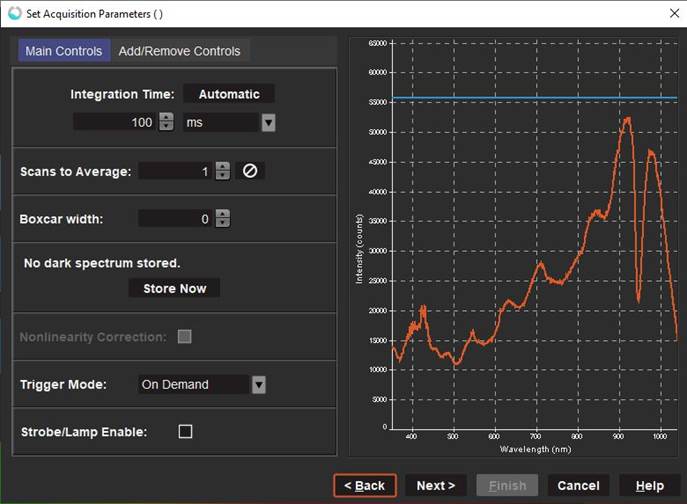
Lower the integration time so the light signal is not saturating (maxing-out) the system. The blue horizontal line on the graph represents about 85% of saturation and is a good target for your maximum signal.
If lowering integration time is not enough, attenuate the light source:
- Use a built‑in attenuator if available
- Use an inline attenuator (FVA-UV) if needed
- As a last resort, introduce temporary optical attenuation by placing a low‑lint disposable wipe between the sample holder and the spectrometer, taking care not to disturb the setup.
Set Boxcar and Averaging
While in this screen, set the smoothing and averaging parameters.
Set Boxcar to around 5
This is horizontal smoothing, so you will notice the trend getting smoother at higher numbers.
Too-low will show excessive noise; too-high will mute sharp peaks. 5 – 10 is usually a safe range for UV-VIS units.
Set Averaging to 5-10
Total Scan Time = Integration Time x Averaging
If you are running down at 5ms, you can run 20 averages and still update at 10Hz.
But if you are running way up at 1 sec, 20 averages will take 20 seconds per scan!
Take the Light Reference
Once the signal looks smooth and stays below the blue line, click Next.
This is your Light Reference. With the light on and the blank sample still in place,
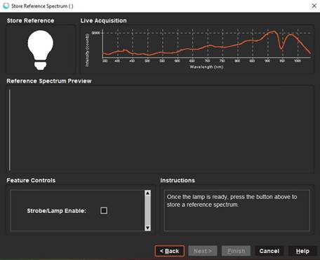
click the white light bulb to store the light the reference, then click Next.
Take the Dark Reference
This is your Dark Reference. Next, block or turn off the light source so no light reaches the spectrometer.
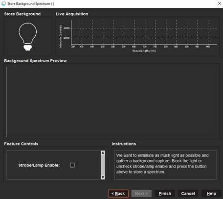
Click the black light bulb to store the dark reference, then click Finish.
Adjust the Absorbance Graph
You’re now in Absorbance mode! A new graph tab labeled Absorbance View will appear.
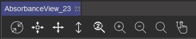
Manually Set Axis Ranges
Click the magnifier with numbers to manually set the graph axes.
- Leave the x‑axis as‑is unless you want to focus on a specific wavelength range
- Set the y‑axis to start around −0.5 and end around 2.0
Auto-Scale for Quick Viewing
After inserting your real sample, use the up/down arrow to auto‑scale the y‑axis based on the current data.
This makes it easy to quickly see changes without altering the wavelength range.
Saving Your Absorbance Data
To save your data, click the gear icon at the top of the graph to open File Saving Parameters.

Set the file location, base name, file type, and saving behavior. Make sure you are saving to a known location on your device. The default single‑scan mode works well for most users.
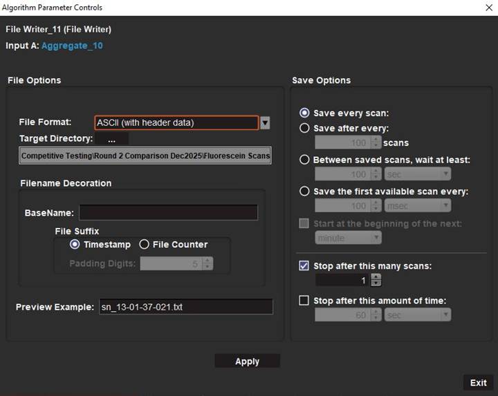
Once you have the parameters set how you want, click Apply and close that window. Now use the download button to save a file based on those parameters; every time you click that will initiate a save.

The file can be opened in Excel or similar program, with the wavelengths in the left column and absorbance values in the right column. If you went through this data saving procedure in the original intensity graph, the data would be intensity values rather than absorbance.
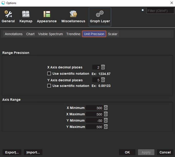
Extra Tip: Precision and Display Options
If you want more control over how your data appears, right‑click inside the graph and open Graph Layer Options. From there, you can adjust decimal precision, font size, colors, and other display settings to match your preferences.
These steps cover the basics of absorbance measurement setup in OceanView. More advanced features such as baselining, strip charts, and peak analysis are available once you are comfortable with the workflow. Stay tuned for future Tech Tips that explore these tools in more depth.